
Lesson 07 · 約 18 分鐘
AI 全景地圖
從 ML 到生成式 AI 的整體脈絡
07 ・ AI 全景地圖:LLM 只是其中一塊
你說「不只物理 AI 和 LLM,別的也想懂」——這份把整片 AI 領土攤開給你看。 好消息:它們大多共用同一套引擎,懂了 LLM,你已經懂了一半。
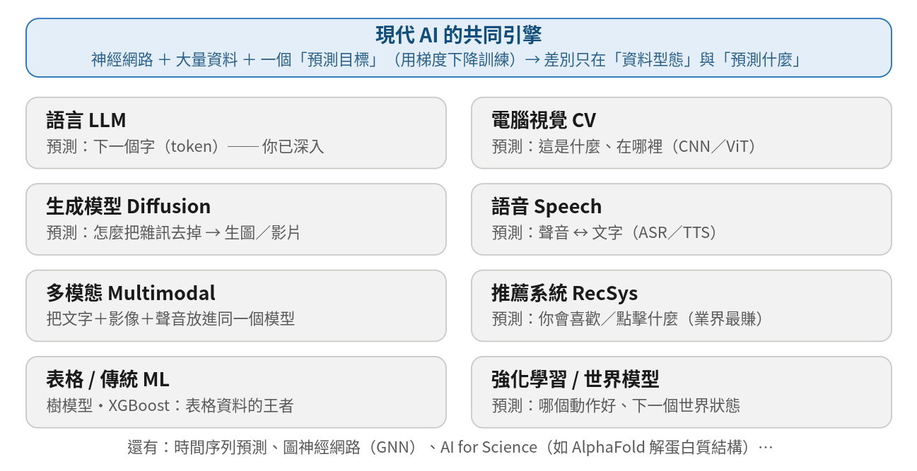
一個關鍵觀念:同一套引擎,不同任務
幾乎所有現代 AI 都是同一個配方:
神經網路 + 大量資料 + 一個「預測目標」,用梯度下降訓練。
差別只在**「吃什麼資料」和「預測什麼」**:
- LLM:預測「下一個字」。
- 電腦視覺:預測「這是什麼、在哪裡」。
- 生成模型(Diffusion):預測「怎麼把雜訊一步步去掉」→ 生成圖片/影片。
- 語音:預測「聲音 ↔ 文字」。
- 推薦系統:預測「你會喜歡/點擊什麼」。
- 強化學習:預測「哪個動作獎勵最高」。
- 世界模型:預測「下一個世界狀態」。
所以你在 code/04 學的反向傳播、code/01 學的注意力、梯度下降——是所有這些領域共用的底層。換領域,主要是換資料和換預測目標,引擎不太變。
各領域速覽(這是什麼/預測什麼/代表例子)
1. 自然語言處理 NLP / 大型語言模型 LLM ── 你已深入
文字。預測下一個字。代表:GPT、Claude、Gemini。→ 見 docs/01。
2. 電腦視覺 Computer Vision
影像與影片。任務有:分類(這是貓還是狗)、偵測(框出物件,如 YOLO)、分割(每個像素屬於什麼)。
架構從 CNN(卷積,擅長抓局部圖樣)走到 ViT(Vision Transformer,把圖切塊當 token,用注意力)。
👉 跑 code/12_cnn_vision.py:先看卷積怎麼當「邊緣偵測器」,再訓練一個小 CNN 把手寫數字辨識到 9 成以上。
3. 生成模型 Generative Models ── 和你關心的 Cosmos 同源
不只判讀,還能「生成」。三大類:
- Diffusion(擴散):學「怎麼把雜訊一步步去成清晰的圖」。Stable Diffusion、影片生成、NVIDIA Cosmos 都是這類。← 現在最主流。
- GAN:兩個網路對抗(一個造假、一個抓假),互相逼強。
- VAE / Autoencoder:學把資料壓縮再還原,順便學到「資料的潛在結構」。
4. 語音 Speech
- ASR(語音轉文字):代表 Whisper。
- TTS(文字轉語音):把字念出來,現在能很自然。
5. 多模態 Multimodal
把文字+影像+聲音放進同一個模型。代表:CLIP(讓圖和文字對齊)、能看圖的 GPT-4V 類模型。VLM(視覺語言模型)就屬這塊。→ 也和 docs/02 的 VLM 對照。
👉 跑 code/16_clip_contrastive.py:用對比學習(InfoNCE)把「圖」和「文」對齊到同一向量空間,看檢索準確率從亂猜爬到 9 成。
6. 推薦系統 Recommendation ── 業界最賺錢的 AI
YouTube/Netflix/電商/廣告背後的引擎,預測「你最可能喜歡/點擊什麼」。技術上常用embedding(把人和物變向量)+ 排序模型。低調但商業價值極高。
👉 跑 code/17_recommender.py:用矩陣分解(協同過濾)讓模型自己從評分模式發現「口味群」,補出沒看過的評分並推薦。
7. 表格資料 / 傳統機器學習 ── 別小看
真實世界大量是表格資料(試算表那種)。這裡梯度提升樹(XGBoost / LightGBM)常常打贏深度學習,而且快、好解釋。Kaggle 表格賽的常勝軍。你做股票/財務分析,這塊超實用。
👉 跑 code/14_tabular_ml.py:比較梯度提升樹 vs 線性基準線、算特徵重要度,並學到「複雜模型不一定贏,要比基準線」的鐵則。
8. 強化學習 RL / 機器人 / 世界模型 ── 你已碰
靠「嘗試+獎勵」學行動。→ 見 code/06(Q-learning)、docs/02、docs/03。
還有(同樣值得知道)
- 時間序列預測:股價、用電、需求預測(你有股票興趣,這塊可玩)。👉 跑
code/13_timeseries_forecast.py:學「照時間切、先比基準線、用 MAE/RMSE」的紀律,AR 自迴歸 vs 笨基準線。 - 圖神經網路 GNN:處理「網路狀」資料——社群關係、分子結構、知識圖。👉 跑
code/15_gnn_from_scratch.py:手刻 GCN,靠訊息傳遞只用 2 個標籤就把整張圖的節點分到正確社群。 - AI for Science:用 AI 解科學難題,如 AlphaFold(預測蛋白質 3D 結構,拿了諾貝爾獎相關肯定)、天氣預報、新材料/新藥探索。
它們怎麼組合起來
真實產品常是好幾塊疊在一起:
- 會看圖的聊天助理 = LLM + 視覺 + 多模態。
- 能畫圖的工具 = LLM 理解你的話 + Diffusion 生成圖。
- 自駕車/機器人 = 視覺(看路)+ 世界模型(預測)+ RL(決策)+ 規劃。
- 電商 = 推薦系統 + 表格 ML + 時間序列。
想往哪鑽?(怎麼用這份學習包接下去)
- 你已有的:LLM(
docs/01+code/01,02,04,05)、RL/世界模型(docs/02,03+code/03,06)。 - 想補生成/Diffusion:它和世界模型同源,是很自然的下一步。
- 想補視覺:從 CNN 入手(fast.ai、CS231n)。
- 想補表格 ML:學 XGBoost/LightGBM,配 Kaggle 練手(對你的股票分析直接有用)。
- 每塊的資源與必讀論文,依難度分層放在
docs/05_進階路線_簡單到大師.md。
一句話收尾:AI 不是很多互不相干的魔法,而是「同一套引擎」套到不同資料與任務上。 你不必每塊都精通;先把引擎吃透(你正在做),再挑有興趣的領域深入,其餘大多能快速看懂。
🛠 跟著做
共 7 支 · 在本機 venv 跑 · 還沒裝環境?
numpy📄 原始碼
"""
08_mini_rag.py
================================
從零做一個「迷你 RAG(檢索增強生成)」——只用 numpy + 標準庫,不需任何模型或網路。
對照講義 docs/00(第 4 站)、docs/05(進階,RAG 論文)。

RAG 是業界最常見的 LLM 應用:「先去你的資料裡找相關段落,再把段落塞給模型回答」,
這樣模型能回答它沒背過的、或最新的、或私有的知識,也比較不會亂編。

完整流程(這支程式把每一步都做出來):
  1. 切塊(chunk):把文件切成一段一段。
  2. 向量化(embed):把每段文字變成一個數字向量。這裡用最經典的 TF-IDF。
  3. 檢索(retrieve):把問題也向量化,用「餘弦相似度」找最像的前 k 段。
  4. 生成(generate):把「問題 + 找到的段落」組成答案。

  ⚠️ 真實 RAG 會把第 2 步的 TF-IDF 換成「神經網路嵌入模型」(語意更強),
     第 4 步的拼接換成「丟給 LLM 寫成流暢回答」。但機制與骨架,就是這支程式這樣。
     先把骨架吃透,換零件就很直覺。

執行:python3 08_mini_rag.py   (只需要 numpy)
"""

import sys
import math
import re
from collections import Counter
import numpy as np

if hasattr(sys.stdout, "reconfigure"):
    sys.stdout.reconfigure(encoding="utf-8")


# 一份小「知識庫」(你可以換成任何你自己的筆記/教材)
KNOWLEDGE_BASE = """\
注意力機制的公式是 softmax(Q乘K轉置除以根號d)乘V。Q代表我在找什麼,K代表我有什麼,V代表我能提供的內容。
因果遮罩讓第i個字只能看到第1到i個字,看不到未來,這是GPT一個字一個字往下生成的關鍵。
預訓練的目標是預測下一個token,損失函數用交叉熵,優化器用AdamW做梯度下降。
後訓練包含SFT監督式微調、RLHF人類回饋強化學習、以及DPO直接偏好優化,把會接話的模型變成聽指令的助理。
LoRA是一種低秩微調方法,只訓練少量新增的低秩矩陣,凍結原本的大模型權重,省記憶體又快。
世界模型學的是預測下一個世界狀態,機器人用它在腦中試走,這叫MPC模型預測控制。
RAG檢索增強生成的做法是先從資料庫找相關段落,再把段落餵給模型回答,能回答私有或最新知識。
量化是把模型權重從32位元浮點數壓成8位元或4位元整數,讓模型更小更快,常見方法有GPTQ和AWQ。
"""


def split_chunks(text):
    """把文件切成一段一段(這裡用句號切;真實系統會用更聰明的切法並控制每塊長度)。"""
    parts = [s.strip() for s in re.split(r"[。\n]", text) if s.strip()]
    return parts


# 停用詞:到處都有、沒鑑別度的字。真實系統也會做這步(去掉雜訊、讓檢索更準)。
STOPWORDS = set("的是在有和與把這那個了嗎呢嗎什麼怎麼如何你我他她它們之就也都會能要可以及以")


def tokenize(s):
    """超簡易斷詞:中文逐字、英數成詞,並濾掉停用詞。真實系統會用 BPE(見 code/05)或神經嵌入。"""
    tokens = re.findall(r"[a-zA-Z0-9]+", s)              # 抓英數詞
    tokens += re.findall(r"[一-鿿]", s)          # 抓中文單字
    return [t.lower() for t in tokens if t not in STOPWORDS]


def build_tfidf(chunks):
    """
    把每個 chunk 變成 TF-IDF 向量。
      TF(詞頻):某詞在這段出現幾次(出現多 = 對這段重要)。
      IDF(逆文件頻率):某詞在越少段落出現 = 越有鑑別度(像「的」到處都有 → 沒鑑別度)。
      TF-IDF = TF × IDF,最後做 L2 正規化方便算餘弦相似度。
    回傳 (向量矩陣 (n_chunks, vocab), 詞->欄位的對照 vocab, idf 向量)。
    """
    docs_tokens = [tokenize(c) for c in chunks]
    vocab = sorted(set(t for toks in docs_tokens for t in toks))
    vidx = {w: i for i, w in enumerate(vocab)}
    N = len(chunks)

    # df:每個詞出現在幾個 chunk
    df = np.zeros(len(vocab))
    for toks in docs_tokens:
        for w in set(toks):
            df[vidx[w]] += 1
    idf = np.log((N + 1) / (df + 1)) + 1.0           # 平滑版 IDF

    mat = np.zeros((N, len(vocab)))
    for i, toks in enumerate(docs_tokens):
        counts = Counter(toks)
        for w, c in counts.items():
            mat[i, vidx[w]] = c * idf[vidx[w]]       # TF × IDF
    # L2 正規化:之後兩向量內積 = 餘弦相似度
    norms = np.linalg.norm(mat, axis=1, keepdims=True)
    mat = mat / np.where(norms == 0, 1, norms)
    return mat, vidx, idf


def embed_query(q, vidx, idf):
    """把問題用同一套 TF-IDF 規則變成向量(只用知識庫學到的詞表與 idf)。"""
    vec = np.zeros(len(vidx))
    counts = Counter(tokenize(q))
    for w, c in counts.items():
        if w in vidx:                                # 沒見過的詞忽略
            vec[vidx[w]] = c * idf[vidx[w]]
    norm = np.linalg.norm(vec)
    return vec / norm if norm > 0 else vec


def retrieve(query, chunks, mat, vidx, idf, k=2):
    """檢索:算問題向量和每段的餘弦相似度,回傳分數最高的前 k 段。"""
    qv = embed_query(query, vidx, idf)
    scores = mat @ qv                                # 因為都正規化過,內積=餘弦相似度
    top = np.argsort(scores)[::-1][:k]
    return [(chunks[i], scores[i]) for i in top]


def generate_answer(query, retrieved):
    """
    「生成」:迷你版本就是把找到的段落組成回答(萃取式)。
    真實 RAG 在這一步會把 query + 段落丟給 LLM,寫成一段流暢的話。
    """
    if not retrieved or retrieved[0][1] == 0:
        return "(知識庫裡找不到相關內容——真實系統這時應誠實說不知道,而不是亂編。)"
    lines = [f"根據知識庫,關於「{query}」:"]
    for i, (chunk, score) in enumerate(retrieved, 1):
        lines.append(f"  [{i}] {chunk}。(相關度 {score:.3f})")
    return "\n".join(lines)


def main():
    chunks = split_chunks(KNOWLEDGE_BASE)
    mat, vidx, idf = build_tfidf(chunks)
    print("=" * 64)
    print(f"知識庫切成 {len(chunks)} 段,詞表大小 {len(vidx)}。")
    print("=" * 64)

    questions = [
        "注意力的公式是什麼?",
        "LoRA 是什麼,有什麼好處?",
        "怎麼讓模型變小變快?",
        "今天天氣如何?",          # 故意問知識庫沒有的,看它會不會誠實
    ]
    for q in questions:
        print(f"\n❓ 問題:{q}")
        retrieved = retrieve(q, chunks, mat, vidx, idf, k=2)
        print(generate_answer(q, retrieved))

    print("\n" + "=" * 64)
    print("這就是 RAG 的完整骨架:切塊 → 向量化 → 檢索 → 生成。")
    print("把 TF-IDF 換成神經嵌入、把拼接換成 LLM,就是你會在業界做的真實 RAG。")


if __name__ == "__main__":
    main()
numpy📄 原始碼
"""
11_mini_diffusion.py
================================
從零做一個「迷你 Diffusion(擴散生成模型)」——只用 numpy,手刻去噪網路 + 反向傳播。
對照講義 docs/07(全景地圖:生成模型)。Diffusion 是 Stable Diffusion、影片生成、
以及 NVIDIA Cosmos(你關心的物理 AI 世界生成)背後的同一套想法。

核心觀念(和 LLM 一樣是「同一套引擎」,只是換了預測目標):
  - 前向過程:對乾淨資料一步步加高斯雜訊,最後變成純雜訊(這步不用學,是固定的)。
  - 反向過程:訓練一個網路,學會「看一個有雜訊的樣本,猜出裡面被加了多少雜訊」。
  - 生成:從純雜訊出發,反覆用網路把雜訊一點點去掉 → 長出一個像訓練資料的新樣本。

這裡的「資料」是 2D 平面上一個圓上的點。訓練後,從雜訊取樣出來的新點,
應該也會落在那個圓附近(半徑接近 2)——代表模型學會了資料的形狀。

執行:python3 11_mini_diffusion.py   (只需要 numpy,約幾秒)
"""

import sys
import numpy as np

if hasattr(sys.stdout, "reconfigure"):
    sys.stdout.reconfigure(encoding="utf-8")

rng = np.random.default_rng(0)


# ──────────────────────────────────────────────────────────────
# 資料:2D 圓上的點(這就是我們要模型學會「生成」的分佈)
# ──────────────────────────────────────────────────────────────
def sample_data(n):
    theta = rng.uniform(0, 2 * np.pi, size=n)
    r = 2.0
    pts = np.stack([r * np.cos(theta), r * np.sin(theta)], axis=1)
    return pts + rng.normal(0, 0.03, size=(n, 2))      # 加一點點厚度


# ──────────────────────────────────────────────────────────────
# 雜訊排程(固定,不用學):betas → alphas → alpha_bar
#   x_t = sqrt(alpha_bar_t)·x_0 + sqrt(1-alpha_bar_t)·eps
# ──────────────────────────────────────────────────────────────
T = 40
betas = np.linspace(1e-4, 0.05, T)
alphas = 1.0 - betas
alpha_bars = np.cumprod(alphas)


# ──────────────────────────────────────────────────────────────
# 去噪網路:一個 2 層 MLP,輸入 [x_t(2) , t正規化(1)],輸出「猜的雜訊」(2)。
# 全部手刻 forward / backward(這就是 PyTorch 幫你自動做的事)。
# ──────────────────────────────────────────────────────────────
H = 128
def init_params():
    return dict(
        W1=rng.normal(0, 0.3, (3, H)), b1=np.zeros(H),
        W2=rng.normal(0, 0.3, (H, H)), b2=np.zeros(H),
        W3=rng.normal(0, 0.3, (H, 2)), b3=np.zeros(2),
    )


def forward(p, X):
    z1 = X @ p["W1"] + p["b1"]; a1 = np.tanh(z1)
    z2 = a1 @ p["W2"] + p["b2"]; a2 = np.tanh(z2)
    out = a2 @ p["W3"] + p["b3"]
    cache = (X, z1, a1, z2, a2)
    return out, cache


def backward(p, cache, dout):
    X, z1, a1, z2, a2 = cache
    grads = {}
    grads["W3"] = a2.T @ dout;            grads["b3"] = dout.sum(0)
    da2 = dout @ p["W3"].T
    dz2 = da2 * (1 - a2 ** 2)             # tanh' = 1 - tanh²
    grads["W2"] = a1.T @ dz2;             grads["b2"] = dz2.sum(0)
    da1 = dz2 @ p["W2"].T
    dz1 = da1 * (1 - a1 ** 2)
    grads["W1"] = X.T @ dz1;              grads["b1"] = dz1.sum(0)
    return grads


# 簡易 Adam 優化器(讓 diffusion 訓練穩定收斂)
class Adam:
    def __init__(self, params, lr=2e-3):
        self.lr = lr
        self.m = {k: np.zeros_like(v) for k, v in params.items()}
        self.v = {k: np.zeros_like(v) for k, v in params.items()}
        self.t = 0

    def step(self, params, grads):
        self.t += 1
        for k in params:
            self.m[k] = 0.9 * self.m[k] + 0.1 * grads[k]
            self.v[k] = 0.999 * self.v[k] + 0.001 * grads[k] ** 2
            mhat = self.m[k] / (1 - 0.9 ** self.t)
            vhat = self.v[k] / (1 - 0.999 ** self.t)
            params[k] -= self.lr * mhat / (np.sqrt(vhat) + 1e-8)


# ──────────────────────────────────────────────────────────────
# 訓練:教網路「看 x_t 與 t,猜出被加的雜訊 eps」
# ──────────────────────────────────────────────────────────────
def train(steps=4000, batch=256):
    p = init_params()
    opt = Adam(p)
    for it in range(steps + 1):
        x0 = sample_data(batch)
        t = rng.integers(0, T, size=batch)                  # 每個樣本隨機挑一個時間步
        ab = alpha_bars[t][:, None]
        eps = rng.normal(0, 1, size=(batch, 2))             # 真正加進去的雜訊(標準答案)
        xt = np.sqrt(ab) * x0 + np.sqrt(1 - ab) * eps       # 前向加噪
        X = np.concatenate([xt, (t[:, None] / T)], axis=1)  # 網路輸入

        pred, cache = forward(p, X)
        diff = pred - eps
        loss = np.mean(diff ** 2)                           # 預測雜訊 vs 真雜訊
        dout = (2.0 / batch) * diff
        grads = backward(p, cache, dout)
        opt.step(p, grads)
        if it % 1000 == 0:
            print(f"  step {it:5d} | loss(預測雜訊的誤差) = {loss:.4f}")
    return p


# ──────────────────────────────────────────────────────────────
# 取樣(生成):從純雜訊出發,反覆去噪(DDPM 反向過程)
# ──────────────────────────────────────────────────────────────
def sample(p, n=2000):
    x = rng.normal(0, 1, size=(n, 2))                       # 從純雜訊開始
    for t in reversed(range(T)):
        tt = np.full((n, 1), t / T)
        eps_pred, _ = forward(p, np.concatenate([x, tt], axis=1))
        beta, alpha, ab = betas[t], alphas[t], alpha_bars[t]
        # 用預測的雜訊,估出這一步去噪後的均值
        mean = (x - beta / np.sqrt(1 - ab) * eps_pred) / np.sqrt(alpha)
        if t > 0:
            x = mean + np.sqrt(beta) * rng.normal(0, 1, size=(n, 2))
        else:
            x = mean
    return x


def main():
    print("=" * 64)
    print("訓練迷你 Diffusion:學會生成『2D 圓上的點』(真實半徑 = 2.0)")
    print("=" * 64)
    p = train()

    print("\n從純雜訊取樣 2000 個新點,看它們長得像不像訓練資料:")
    gen = sample(p)
    radii = np.sqrt((gen ** 2).sum(1))
    print(f"  生成點的平均半徑 = {radii.mean():.3f}(目標 2.0)")
    print(f"  半徑標準差       = {radii.std():.3f}(越小代表越貼合圓)")
    print(f"  落在半徑 1.5~2.5 之間的比例 = {np.mean((radii > 1.5) & (radii < 2.5)) * 100:.1f}%")
    print()
    print("解讀:從一堆隨機雜訊出發,網路靠『反覆去噪』把它們推回圓上——")
    print("這就是 Stable Diffusion 生圖、Cosmos 生世界的同一套機制,只是這裡資料是 2D 點。")


if __name__ == "__main__":
    main()
torchnumpyscikit-learn📄 原始碼
"""
12_cnn_vision.py
================================
電腦視覺入門:卷積神經網路(CNN)。對照講義 docs/07(全景地圖:電腦視覺)。
分兩部分:
  A) 【numpy】卷積到底在幹嘛——把卷積當成「特徵偵測器」,親手對一張數字圖做邊緣偵測。
  B) 【PyTorch】訓練一個小 CNN 辨識手寫數字(用 sklearn 內建的 8x8 digits,免下載)。

核心直覺:
  - 卷積 = 拿一個小「核(kernel)」在圖上滑動做加權求和。不同的核偵測不同特徵
    (垂直邊、水平邊、角…)。CNN 的厲害在於:這些核不是人設計的,是「訓練學出來的」。
  - 池化(pooling)= 把圖縮小、保留最強反應,讓特徵有「平移容忍度」、也省計算。
  - 多層疊起來:淺層抓邊角、深層組合成形狀/物件——和注意力一樣是「同一套引擎」,
    只是這裡的歸納偏好是「局部 + 平移不變」,特別適合影像。

執行:python3 12_cnn_vision.py
需要:numpy、scikit-learn(取資料)、PyTorch(B 部分訓練)。
"""

import sys
import numpy as np

if hasattr(sys.stdout, "reconfigure"):
    sys.stdout.reconfigure(encoding="utf-8")


# ──────────────────────────────────────────────────────────────
# A) 純 numpy:卷積 = 特徵偵測器
# ──────────────────────────────────────────────────────────────
def conv2d(img, kernel):
    """最樸素的 2D 卷積(valid,無填充):核在圖上滑動做加權求和。"""
    kh, kw = kernel.shape
    H, W = img.shape
    out = np.zeros((H - kh + 1, W - kw + 1))
    for i in range(out.shape[0]):
        for j in range(out.shape[1]):
            out[i, j] = np.sum(img[i:i + kh, j:j + kw] * kernel)
    return out


def ascii_art(img):
    """把灰階小圖印成 ASCII,肉眼看得到形狀。"""
    chars = " .:-=+*#%@"
    lo, hi = img.min(), img.max()
    norm = (img - lo) / (hi - lo + 1e-9)
    lines = []
    for row in norm:
        lines.append("".join(chars[int(v * (len(chars) - 1))] for v in row))
    return "\n".join(lines)


def demo_convolution():
    from sklearn.datasets import load_digits
    digits = load_digits()
    img = digits.images[0]                    # 一張 8x8 的手寫「0」

    print("=" * 64)
    print("A) 卷積是特徵偵測器(純 numpy)")
    print("=" * 64)
    print("原圖(手寫數字,越亮筆畫越濃):")
    print(ascii_art(img))

    # 兩個人工設計的核:Sobel 垂直/水平邊緣偵測器
    sobel_v = np.array([[-1, 0, 1], [-2, 0, 2], [-1, 0, 1]])    # 偵測垂直邊
    sobel_h = np.array([[-1, -2, -1], [0, 0, 0], [1, 2, 1]])    # 偵測水平邊

    print("\n經『垂直邊偵測核』後(亮處 = 偵測到垂直邊):")
    print(ascii_art(np.abs(conv2d(img, sobel_v))))
    print("\n經『水平邊偵測核』後(亮處 = 偵測到水平邊):")
    print(ascii_art(np.abs(conv2d(img, sobel_h))))
    print("\n→ 同一張圖,不同的核挑出不同特徵。CNN 把這些核變成『可訓練的參數』,")
    print("  讓模型自己學出『對辨識數字最有用的核』。\n")


# ──────────────────────────────────────────────────────────────
# B) PyTorch:訓練一個小 CNN 辨識手寫數字
# ──────────────────────────────────────────────────────────────
def train_cnn():
    import torch
    import torch.nn as nn
    from sklearn.datasets import load_digits
    from sklearn.model_selection import train_test_split

    torch.manual_seed(0)
    print("=" * 64)
    print("B) 訓練小 CNN 辨識手寫數字(PyTorch)")
    print("=" * 64)

    digits = load_digits()
    X = digits.images / 16.0                                  # (1797, 8, 8) 正規化到 0~1
    y = digits.target
    Xtr, Xte, ytr, yte = train_test_split(X, y, test_size=0.2, random_state=0)

    Xtr = torch.tensor(Xtr, dtype=torch.float32).unsqueeze(1)  # (N,1,8,8):1 個顏色通道
    Xte = torch.tensor(Xte, dtype=torch.float32).unsqueeze(1)
    ytr = torch.tensor(ytr, dtype=torch.long)
    yte = torch.tensor(yte, dtype=torch.long)

    model = nn.Sequential(
        nn.Conv2d(1, 8, 3, padding=1), nn.ReLU(), nn.MaxPool2d(2),   # 8x8 -> 8 張 4x4 特徵圖
        nn.Conv2d(8, 16, 3, padding=1), nn.ReLU(), nn.MaxPool2d(2),  # -> 16 張 2x2
        nn.Flatten(),
        nn.Linear(16 * 2 * 2, 10),                                  # -> 10 個數字的分數
    )
    n_params = sum(p.numel() for p in model.parameters())
    print(f"CNN 參數量:{n_params/1e3:.1f}K,訓練樣本 {len(Xtr)}、測試 {len(Xte)}")

    opt = torch.optim.Adam(model.parameters(), lr=1e-3)
    loss_fn = nn.CrossEntropyLoss()
    batch = 64
    for epoch in range(1, 16):
        model.train()
        perm = torch.randperm(len(Xtr))                      # 每個 epoch 打亂順序
        last_loss = 0.0
        for s in range(0, len(Xtr), batch):                  # mini-batch:分小批多次更新
            idx = perm[s:s + batch]
            opt.zero_grad()
            loss = loss_fn(model(Xtr[idx]), ytr[idx])
            loss.backward()
            opt.step()
            last_loss = loss.item()
        if epoch % 3 == 0:
            model.eval()
            with torch.no_grad():
                acc = (model(Xte).argmax(1) == yte).float().mean().item()
            print(f"  epoch {epoch:2d} | train loss {last_loss:.3f} | 測試準確率 {acc*100:.1f}%")

    print("\n→ 一個幾千參數的小 CNN,就能把 8x8 手寫數字辨識到 9 成以上。")
    print("  把資料換成更大的彩色圖、把網路加深,就是 ResNet/ViT 那條路(docs/07)。")


def main():
    demo_convolution()
    try:
        train_cnn()
    except ImportError as e:
        print(f"(跳過 B 部分:缺少套件 {e.name}。安裝 torch 與 scikit-learn 後可跑訓練。)")


if __name__ == "__main__":
    main()
scikit-learnnumpy📄 原始碼
"""
14_tabular_ml.py
================================
表格資料機器學習(tabular ML)——別小看這塊:真實世界一大半是試算表那種資料,
而這裡「梯度提升樹(XGBoost / LightGBM)常常打贏深度學習」,又快又好解釋。
你做股票/財務分析(一堆數值欄位 → 預測漲跌),正是典型的表格 ML 問題。
對照講義 docs/07(全景地圖:表格資料 / 傳統機器學習)。

這支程式示範一個專業的表格 ML 流程:
  1. 切 train/test,公平比較三種模型:
       - 邏輯回歸(線性基準線)
       - 隨機森林(很多棵樹投票)
       - 梯度提升樹(HistGradientBoosting,和 XGBoost/LightGBM 同一套想法)
  2. 用 accuracy 與 ROC AUC 評估(AUC 對不平衡資料更可靠)。
  3. 算「特徵重要度」:哪些欄位最影響預測——這對金融/醫療的可解釋性極重要。

⚠️ 這裡用 sklearn 內建的乳癌診斷資料(30 個數值特徵,免下載)示範方法。
   換成你自己的股票特徵表(同樣是「數值欄位 → 標籤」),流程一模一樣。
   xgboost / lightgbm 沒裝也沒關係:HistGradientBoosting 就是同類,效能接近、API 類似。

執行:python3 14_tabular_ml.py    需要:scikit-learn、numpy
"""

import os
import sys
import numpy as np

# 避免 sklearn 平行後端在 Windows 上找 CPU 核數時跳的無害警告
os.environ.setdefault("LOKY_MAX_CPU_COUNT", "4")

if hasattr(sys.stdout, "reconfigure"):
    sys.stdout.reconfigure(encoding="utf-8")


def main():
    from sklearn.datasets import load_breast_cancer
    from sklearn.model_selection import train_test_split
    from sklearn.linear_model import LogisticRegression
    from sklearn.ensemble import RandomForestClassifier, HistGradientBoostingClassifier
    from sklearn.preprocessing import StandardScaler
    from sklearn.metrics import accuracy_score, roc_auc_score
    from sklearn.inspection import permutation_importance

    data = load_breast_cancer()
    X, y = data.data, data.target           # (569, 30) 個數值特徵,標籤 0/1
    feat_names = data.feature_names
    Xtr, Xte, ytr, yte = train_test_split(X, y, test_size=0.25,
                                          random_state=0, stratify=y)

    print("=" * 64)
    print(f"表格資料:{X.shape[0]} 筆、{X.shape[1]} 個特徵;訓練 {len(Xtr)} / 測試 {len(Xte)}")
    print("=" * 64)

    # 線性模型對尺度敏感,先標準化(樹模型不需要,但統一處理不影響)
    scaler = StandardScaler().fit(Xtr)
    Xtr_s, Xte_s = scaler.transform(Xtr), scaler.transform(Xte)

    models = {
        "邏輯回歸(線性基準線)  ": (LogisticRegression(max_iter=5000), Xtr_s, Xte_s),
        "隨機森林              ": (RandomForestClassifier(n_estimators=200, random_state=0, n_jobs=1), Xtr, Xte),
        "梯度提升樹(HistGB)★   ": (HistGradientBoostingClassifier(random_state=0), Xtr, Xte),
    }

    print("\n模型比較(測試集):")
    best_name, best_model, best_auc = None, None, -1
    for name, (model, xt, xv) in models.items():
        model.fit(xt, ytr)
        pred = model.predict(xv)
        proba = model.predict_proba(xv)[:, 1]
        acc = accuracy_score(yte, pred)
        auc = roc_auc_score(yte, proba)
        print(f"  {name} | accuracy={acc:.3f} | ROC AUC={auc:.4f}")
        if auc > best_auc:
            best_name, best_model, best_auc, best_X = name, model, auc, xv

    print(f"\n最佳模型:{best_name.strip()}(AUC={best_auc:.4f})")
    if "邏輯回歸" in best_name:
        print("  👀 注意:這份資料近乎『線性可分』,所以線性基準線就贏了——")
        print("     這正是『一定要比基準線』的活教材:別預設複雜模型一定比較好。")

    # 特徵重要度(permutation importance:打亂某欄看分數掉多少 → 適用任何模型)
    print("\n哪些特徵最重要(permutation importance,前 6 名):")
    r = permutation_importance(best_model, best_X, yte, n_repeats=10, random_state=0, n_jobs=1)
    order = np.argsort(r.importances_mean)[::-1][:6]
    for i in order:
        print(f"  {feat_names[i]:<28} 重要度 {r.importances_mean[i]:.4f}")

    print("\n" + "=" * 64)
    print("重點:")
    print("  1. 表格問題上,梯度提升樹通常是『先試的第一個強模型』,在多數真實資料贏過神經網路;")
    print("     但不是萬靈丹——本例這種近線性資料,簡單的邏輯回歸就很強。")
    print("  2. 所以一定要先比基準線(這裡邏輯回歸),確認複雜模型真的有加值,否則白忙。")
    print("  3. 特徵重要度讓你能跟別人解釋『模型為什麼這樣判斷』——金融/醫療超需要。")
    print("  把這套換到你的股票特徵表(本益比、成交量、技術指標…→ 漲/跌),流程一樣。")


if __name__ == "__main__":
    try:
        main()
    except ImportError as e:
        print(f"需要 scikit-learn:pip install scikit-learn(缺 {e.name})")
numpy📄 原始碼
"""
15_gnn_from_scratch.py
================================
圖神經網路(GNN)入門——處理「網路狀」資料:社群關係、分子結構、知識圖譜。
對照講義 docs/07(全景地圖:圖神經網路)。只用 numpy,手刻一個 2 層 GCN + 反向傳播。

核心觀念:「訊息傳遞(message passing)」。
  每個節點的新表示 = 把自己 + 鄰居的特徵做加權平均,再過一個線性層與非線性。
  疊兩層 → 每個節點就「看得到兩跳以內」的鄰居資訊。
  這和注意力『聚合其他位置的資訊』是同一個家族,只是聚合範圍由「圖的邊」決定。

GCN 一層的公式(Kipf & Welling):
    H' = ReLU( Â · H · W )
  其中 Â = D^(-1/2) (A + I) D^(-1/2):加上自環、再做對稱正規化的鄰接矩陣。

任務(半監督節點分類):一張「兩個社群」的圖,只告訴模型每群各 1 個節點的標籤,
看它能不能把其餘節點也正確分到兩群——這正是 GNN 經典的「空手道俱樂部」式問題。

執行:python3 15_gnn_from_scratch.py    (只需要 numpy)
"""

import sys
import numpy as np

if hasattr(sys.stdout, "reconfigure"):
    sys.stdout.reconfigure(encoding="utf-8")

rng = np.random.default_rng(1)


def build_graph():
    """兩個社群、各 5 個節點,群內密集相連、群間只有一條橋。"""
    n = 10
    A = np.zeros((n, n))
    group0 = [0, 1, 2, 3, 4]
    group1 = [5, 6, 7, 8, 9]
    for g in (group0, group1):
        for i in g:
            for j in g:
                if i != j:
                    A[i, j] = 1
    A[4, 5] = A[5, 4] = 1            # 兩群之間唯一的橋
    labels = np.array([0, 0, 0, 0, 0, 1, 1, 1, 1, 1])
    return A, labels


def normalize_adj(A):
    """Â = D^(-1/2) (A + I) D^(-1/2):加自環 + 對稱正規化(讓鄰居加權平均尺度穩定)。"""
    A_hat = A + np.eye(A.shape[0])
    deg = A_hat.sum(1)
    d_inv_sqrt = 1.0 / np.sqrt(deg)
    return d_inv_sqrt[:, None] * A_hat * d_inv_sqrt[None, :]


def softmax(z):
    z = z - z.max(1, keepdims=True)
    e = np.exp(z)
    return e / e.sum(1, keepdims=True)


def main():
    A, labels = build_graph()
    n = A.shape[0]
    Ahat = normalize_adj(A)
    X = np.eye(n)                       # 沒有特徵時,用 one-hot 當每個節點的初始特徵

    # 半監督:只給每群 1 個節點當「已知標籤」
    train_mask = np.zeros(n, dtype=bool)
    train_mask[[0, 9]] = True           # 節點 0(群0)、節點 9(群1)
    y_onehot = np.zeros((n, 2)); y_onehot[np.arange(n), labels] = 1

    # 2 層 GCN 參數
    h = 8
    W1 = rng.normal(0, 0.5, (n, h))
    W2 = rng.normal(0, 0.5, (h, 2))

    print("=" * 64)
    print("半監督節點分類:只告訴模型節點 0 屬群0、節點 9 屬群1,其餘要它自己分。")
    print("=" * 64)

    lr = 0.2
    for step in range(201):
        # ── 前向 ──
        Q = Ahat @ X                    # 預先聚合(X 固定,可重用)
        U = Q @ W1                      # (n, h)
        H1 = np.maximum(U, 0)           # ReLU
        P = Ahat @ H1
        Z = P @ W2                      # (n, 2) logits
        probs = softmax(Z)

        # ── 損失:只在「已知標籤」的節點上算交叉熵 ──
        m = train_mask.sum()
        loss = -np.sum(y_onehot[train_mask] * np.log(probs[train_mask] + 1e-9)) / m

        # ── 反向傳播(手算鏈鎖律)──
        dZ = (probs - y_onehot) * train_mask[:, None] / m   # 未標註節點不貢獻梯度
        dW2 = P.T @ dZ
        dP = dZ @ W2.T
        dH1 = Ahat @ dP                 # P = Ahat·H1(Ahat 對稱,故 Ahat.T = Ahat)
        dU = dH1 * (U > 0)              # ReLU 的梯度
        dW1 = Q.T @ dU

        W1 -= lr * dW1
        W2 -= lr * dW2

        if step % 40 == 0:
            pred = probs.argmax(1)
            acc_all = (pred == labels).mean()
            print(f"  step {step:3d} | loss={loss:.4f} | 全部節點分對比例={acc_all*100:.0f}%")

    pred = softmax(Ahat @ np.maximum(Ahat @ X @ W1, 0) @ W2).argmax(1)
    print("\n每個節點的預測群別(真值:0~4 是群0、5~9 是群1):")
    print("  節點:", " ".join(f"{i}" for i in range(n)))
    print("  預測:", " ".join(f"{p}" for p in pred))
    print("  真值:", " ".join(f"{l}" for l in labels))
    print(f"\n只靠 2 個標籤 + 圖結構,就把 {(pred==labels).mean()*100:.0f}% 的節點分對了。")
    print("關鍵:訊息沿著『邊』傳遞——同群密集相連,標籤資訊就在群內擴散開。")
    print("放大版:分子性質預測、詐騙帳號偵測、推薦的圖譜、知識圖推理,都是這套。")


if __name__ == "__main__":
    main()
torchnumpy📄 原始碼
"""
16_clip_contrastive.py
================================
多模態與對比學習(contrastive learning)入門——CLIP 把「圖」和「文字」對齊到同一個
向量空間的核心想法。對照講義 docs/07(全景地圖:多模態)。用 PyTorch(autograd)實作。

核心觀念:對比學習 + InfoNCE 損失。
  - 兩個編碼器:一個把「圖」變向量、一個把「文字」變向量,投影到同一個空間。
  - 訓練目標:讓「配對的圖文」相似度高、「不配對的」相似度低。
  - 做法:一個 batch 有 N 對圖文,算 N×N 的相似度矩陣,
          要求「對角線(正確配對)最大」——等於在每一列做 N 選 1 的分類(InfoNCE)。
  - 學成後:給一段文字,就能用相似度去「檢索」最相關的圖(反之亦然)。零樣本分類也是這樣來的。

這裡用「合成的圖/文特徵」(各自從同一個隱含概念加雜訊投影而來)示範機制;
真實 CLIP 把兩個編碼器換成影像 CNN/ViT 與文字 Transformer,資料是幾億組網路圖文對。

執行:python3 16_clip_contrastive.py    需要:PyTorch
"""

import sys
import numpy as np

if hasattr(sys.stdout, "reconfigure"):
    sys.stdout.reconfigure(encoding="utf-8")


def make_paired_data(n, latent_dim=6, img_dim=32, txt_dim=24, seed=0):
    """
    造 n 對「圖、文」特徵:每一對有自己獨一無二的隱含向量,
    再各自被不同的固定隨機投影 + 雜訊弄成「圖」與「文」兩種表面長相。
    模型要學會「跨過不同模態的表面差異,認出這一張圖配的是哪一段文字」。
    (注意:投影矩陣 Wi/Wt 固定,所以訓練/測試的圖↔文對應關係一致、可學。)
    """
    rng = np.random.default_rng(seed)
    fixed = np.random.default_rng(999)                    # 固定的投影矩陣(跨 train/test 一致)
    Wi = fixed.normal(0, 1, (latent_dim, img_dim))
    Wt = fixed.normal(0, 1, (latent_dim, txt_dim))
    latent = rng.normal(0, 1, (n, latent_dim))            # 每對一個獨立隱向量
    img = latent @ Wi + rng.normal(0, 0.3, (n, img_dim))  # 投影到「圖」空間 + 雜訊
    txt = latent @ Wt + rng.normal(0, 0.3, (n, txt_dim))  # 投影到「文」空間 + 雜訊
    return img.astype(np.float32), txt.astype(np.float32), latent


def main():
    import torch
    import torch.nn as nn
    import torch.nn.functional as F
    torch.manual_seed(0)

    img_dim, txt_dim, shared = 32, 24, 16
    img_tr, txt_tr, _ = make_paired_data(512, seed=0)
    img_te, txt_te, _ = make_paired_data(128, seed=1)
    img_tr, txt_tr = torch.tensor(img_tr), torch.tensor(txt_tr)
    img_te, txt_te = torch.tensor(img_te), torch.tensor(txt_te)

    # 兩個「編碼器」(這裡用兩層 MLP;真實 CLIP 是 CNN/ViT 與 Transformer)
    img_enc = nn.Sequential(nn.Linear(img_dim, 32), nn.ReLU(), nn.Linear(32, shared))
    txt_enc = nn.Sequential(nn.Linear(txt_dim, 32), nn.ReLU(), nn.Linear(32, shared))
    temperature = 0.07

    def retrieval_acc(ie, te):
        """圖→文 top-1 檢索準確率:每張圖找最相似的文字,是不是它的正確配對。"""
        with torch.no_grad():
            ze = F.normalize(img_enc(ie), dim=1)
            zt = F.normalize(txt_enc(te), dim=1)
            sim = ze @ zt.T
            pred = sim.argmax(1)
            return (pred == torch.arange(len(ie))).float().mean().item()

    print("=" * 64)
    print("對比學習(CLIP 式):把圖與文對齊到同一個向量空間")
    print("=" * 64)
    print(f"訓練前 圖→文 檢索準確率(亂猜約 {100/len(img_te):.1f}%):{retrieval_acc(img_te, txt_te)*100:.1f}%")

    params = list(img_enc.parameters()) + list(txt_enc.parameters())
    opt = torch.optim.Adam(params, lr=1e-3)
    n = len(img_tr)
    for epoch in range(1, 31):
        perm = torch.randperm(n)
        for s in range(0, n, 128):
            idx = perm[s:s + 128]
            ze = F.normalize(img_enc(img_tr[idx]), dim=1)
            zt = F.normalize(txt_enc(txt_tr[idx]), dim=1)
            logits = ze @ zt.T / temperature              # (B, B) 相似度矩陣
            targets = torch.arange(len(idx))              # 正確配對在對角線
            # InfoNCE:圖→文 與 文→圖 兩個方向的交叉熵
            loss = (F.cross_entropy(logits, targets) +
                    F.cross_entropy(logits.T, targets)) / 2
            opt.zero_grad(); loss.backward(); opt.step()
        if epoch % 10 == 0:
            print(f"  epoch {epoch:2d} | InfoNCE loss {loss.item():.3f} | "
                  f"測試檢索準確率 {retrieval_acc(img_te, txt_te)*100:.1f}%")

    print("\n→ 從『亂猜』到能高準確率地用文字找出對應的圖(反之亦然)。")
    print("  CLIP 就是這樣學會圖文對齊,進而做零樣本分類、文字搜圖、給生成模型當條件。")


if __name__ == "__main__":
    try:
        main()
    except ImportError as e:
        print(f"需要 PyTorch:pip install torch(缺 {e.name})")
numpy📄 原始碼
"""
17_recommender.py
================================
推薦系統入門——YouTube / Netflix / 電商 / 廣告背後的引擎,業界最賺錢的 AI 之一。
對照講義 docs/07(全景地圖:推薦系統)。只用 numpy,全部手刻。

核心方法:協同過濾的「矩陣分解(Matrix Factorization)」。
  想法:每個使用者、每個物品,各用一個「隱向量(latent vector)」表示。
        某人對某物的評分 ≈ 兩個隱向量的內積(口味越對盤、分數越高)。
        我們只看「已知的評分」反推這些隱向量,就能預測「沒看過的格子」→ 拿來推薦。

這正是 embedding 的威力:把「人」和「物」都變成向量,關係用幾何(內積/距離)表達——
和 LLM 的詞向量、CLIP 的圖文對齊是同一個思想。

執行:python3 17_recommender.py    (只需要 numpy)
"""

import sys
import numpy as np

if hasattr(sys.stdout, "reconfigure"):
    sys.stdout.reconfigure(encoding="utf-8")

rng = np.random.default_rng(0)


# 一個 6 使用者 × 6 電影 的評分表(1~5 星,0 = 還沒看過)
# 設計成兩種口味:前 3 部偏「動作」、後 3 部偏「文藝」
USERS = ["小明", "小華", "小美", "阿強", "阿芳", "老王"]
ITEMS = ["動作A", "動作B", "動作C", "文藝D", "文藝E", "文藝F"]
R = np.array([
    [5, 5, 4, 1, 0, 1],   # 小明:愛動作
    [4, 0, 5, 1, 1, 0],   # 小華:愛動作(有缺值)
    [5, 4, 0, 0, 1, 1],   # 小美:愛動作
    [1, 0, 1, 5, 4, 5],   # 阿強:愛文藝
    [0, 1, 1, 4, 5, 4],   # 阿芳:愛文藝
    [1, 1, 0, 5, 4, 0],   # 老王:愛文藝(有缺值)
], dtype=float)


def train_mf(R, k=2, steps=2000, lr=0.02, reg=0.05):
    """
    矩陣分解:找 P (使用者×k) 與 Q (物品×k),讓 P·Qᵀ 逼近『已知』的評分。
    只對「有評分(非 0)」的格子算誤差與梯度(缺值不參與訓練)。
    """
    n_users, n_items = R.shape
    P = rng.normal(0, 0.1, (n_users, k))      # 使用者隱向量
    Q = rng.normal(0, 0.1, (n_items, k))      # 物品隱向量
    mask = R > 0                              # 哪些格子有評分

    for step in range(steps + 1):
        pred = P @ Q.T
        err = (R - pred) * mask               # 只看有評分的誤差
        # 梯度下降(含 L2 正則化防過擬合):
        P += lr * (err @ Q - reg * P)
        Q += lr * (err.T @ P - reg * Q)
        if step % 500 == 0:
            rmse = np.sqrt((err ** 2).sum() / mask.sum())
            print(f"  step {step:4d} | 已知評分的 RMSE = {rmse:.4f}")
    return P, Q


def main():
    print("=" * 64)
    print("原始評分表(0 = 還沒看過,要預測的就是這些格子)")
    print("=" * 64)
    header = "        " + "".join(f"{it:>7}" for it in ITEMS)
    print(header)
    for u, row in zip(USERS, R):
        print(f"{u:>6}  " + "".join(f"{v:7.0f}" for v in row))

    print("\n訓練矩陣分解(把每人、每片壓成 2 維隱向量)...")
    P, Q = train_mf(R, k=2)

    pred = P @ Q.T
    print("\n" + "=" * 64)
    print("補完後的預測評分表(█ 標出『原本沒看過、現在預測』的格子)")
    print("=" * 64)
    print(header)
    for i, (u, row) in enumerate(zip(USERS, pred)):
        cells = []
        for j, v in enumerate(row):
            mark = "█" if R[i, j] == 0 else " "
            cells.append(f"{v:6.1f}{mark}")
        print(f"{u:>6}  " + "".join(cells))

    # 給每個人推薦「沒看過、且預測分數最高」的一部
    print("\n推薦(每人挑沒看過裡預測最高分的一部):")
    for i, u in enumerate(USERS):
        unseen = np.where(R[i] == 0)[0]
        if len(unseen) == 0:
            continue
        best = unseen[np.argmax(pred[i, unseen])]
        print(f"  {u} → 推薦《{ITEMS[best]}》(預測 {pred[i, best]:.1f} 星)")

    print("\n" + "=" * 64)
    print("觀察:模型自己『發現』了動作派與文藝派兩群人,並據此補出缺的評分。")
    print("這就是協同過濾:沒用到任何電影內容,只靠『大家的評分模式』學出口味。")
    print("放大版:把 k 加大、用神經網路取代內積、加入內容特徵,就是 YouTube/Netflix 的推薦引擎。")


if __name__ == "__main__":
    main()